Introduction to the Catalog classes in orpheus

In this notebooks we introduce the different tracer categories in orpheus and how to construct reduced catalogs.

Basics

Currently, in orpheus we have implemented the following classes for tracer catalogs:

The Catalog class

This is the parent class from which the more specific catalog classes are derived. It only requires the spatial positions of the data of any catalog and contains the implementations for common operations, such as the reduction of catalogs in pixels, the creation of hierarchical spatial hashes, as well as the empirical estimation of anglular masks.

The ScalarTracerCatalog class

This is what you want to use for scalar tracers, such as the weak lensing convergence field. In case you really only want to use (weighted) number counts you can set the tracer to equal to unity.

The SpinTracerCatalog class

This is what you want to use for tracers with a directional dependence, such as the spin-2 weak lensing shear field. In case you really only want to use (weighted) number counts you can set the tracer to equal to unity. The spin of the (complex-valued) tracer is explicitly passed via the spin attribute.

from astropy.table import Table
import numpy as np
from matplotlib import pyplot as plt

import orpheus

Obtaining a realistic mock shape catalog

We will run this notebook using a mocks shape catalog from the SLICS ensemble. First, let us download this catalog and read in its contents.

Note: If you want to run the notebook yourself, you need to update the savepath_SLICS variable.

catname = "GalCatalog_LOS1.fits"
path_to_SLICS = "http://cuillin.roe.ac.uk/~jharno/SLICS/MockProducts/KiDS450/" + catname
savepath_SLICS = "/vol/euclidraid4/data/lporth/HigherOrderLensing/Mocks/SLICS_KiDS450/"

!wget {path_to_SLICS} -P {savepath_SLICS}

slicscat = Table.read(savepath_SLICS + catname)
print(slicscat.keys())

['x_arcmin', 'y_arcmin', 'z_spectroscopic', 'z_photometric', 'shear1', 'shear2', 'eps_obs1', 'eps_obs2']

WARNING: UnitsWarning: 'UNKNOWN' did not parse as fits unit: At col 0, Unit 'UNKNOWN' not supported by the FITS standard.  If this is meant to be a custom unit, define it with 'u.def_unit'. To have it recognized inside a file reader or other code, enable it with 'u.add_enabled_units'. For details, see https://docs.astropy.org/en/latest/units/combining_and_defining.html [astropy.units.core]
WARNING: UnitsWarning: 'UNKNOWN' did not parse as fits unit: At col 0, Unit 'UNKNOWN' not supported by the FITS standard.  If this is meant to be a custom unit, define it with 'u.def_unit'. To have it recognized inside a file reader or other code, enable it with 'u.add_enabled_units'. For details, see https://docs.astropy.org/en/latest/units/combining_and_defining.html [astropy.units.core]

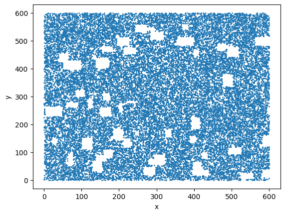
To make things slightly more realistic, let us apply a simplistic angular survey mask where we cut out a bunch of poissonian distributed rectangular shapes of varying sizes

nmask = 50
length_mean = 30
lenght_std = 10
rseed = 42

sx = 600*np.random.rand(nmask)
sy = 600*np.random.rand(nmask)
np.random.seed(rseed)
lx = np.abs(np.random.normal(loc=length_mean,scale=lenght_std,size=nmask))
ly = np.abs(np.random.normal(loc=length_mean,scale=lenght_std,size=nmask))

unmasked = np.ones(len(slicscat['x_arcmin']), dtype=bool)
for imask in range(nmask):
    nextmask = np.ones(len(slicscat['x_arcmin']), dtype=bool)
    nextmask *= (slicscat['x_arcmin']>sx[imask]) * (slicscat['x_arcmin']<(sx[imask]+lx[imask]))
    nextmask *= (slicscat['y_arcmin']>sy[imask]) * (slicscat['y_arcmin']<(sy[imask]+ly[imask]))
    unmasked *= ~nextmask

plt.scatter(slicscat['x_arcmin'][unmasked][::100],slicscat['y_arcmin'][unmasked][::100],s=1)
plt.xlabel('x')
plt.ylabel('y')
plt.show()

Initializing a SpinTracerCatalog instance

As we are dealing with an ellipticity catalog, we need to use the SpinTracerCatalog class and set the value of spin to two.

shapecat = orpheus.SpinTracerCatalog(spin=2,
                                     pos1=slicscat["x_arcmin"][unmasked],
                                     pos2=slicscat["y_arcmin"][unmasked],
                                     tracer_1=slicscat["shear1"][unmasked],
                                     tracer_2=slicscat["shear2"][unmasked])

Looking at the __dict__ of the instance, we see that there are a bunch of more attributes have been allocated. Many of those can be set adjusted in the __init__ and are directly inherited from the parent Catalog class. But let’s keep things simple here.

for i, (k, v) in enumerate(shapecat.__dict__.items()):
    if isinstance(v,np.ndarray):
        print(k,v.shape)
    else:
        print(k,v)

pos1 (2742332,)
pos2 (2742332,)
weight (2742332,)
zbins (2742332,)
ngal 2742332
nbinsz 1
isinner (2742332,)
units_pos1 None
units_pos2 None
geometry flat2d
mask None
zbins_mean None
zbins_std None
min1 1.0337681e-05
min2 4.8615038e-05
max1 599.99976
max2 599.99988
len1 599.999749662319
len2 599.9998313849619
spatialhash None
hasspatialhash False
index_matcher None
pixs_galind_bounds None
pix_gals None
pix1_start None
pix1_d None
pix1_n None
pix2_start None
pix2_d None
pix2_n None
patchinds None
assign_methods {'NGP': 0, 'CIC': 1, 'TSC': 2}
library_path /users/lporth/anaconda3/envs/orpheus_devel/lib/python3.12/site-packages
clib <CDLL '/users/lporth/anaconda3/envs/orpheus_devel/lib/python3.12/site-packages/orpheus_clib.cpython-312-x86_64-linux-gnu.so', handle 37ae8e20 at 0x71192f68d2b0>
tracer_1 (2742332,)
tracer_2 (2742332,)
spin 2

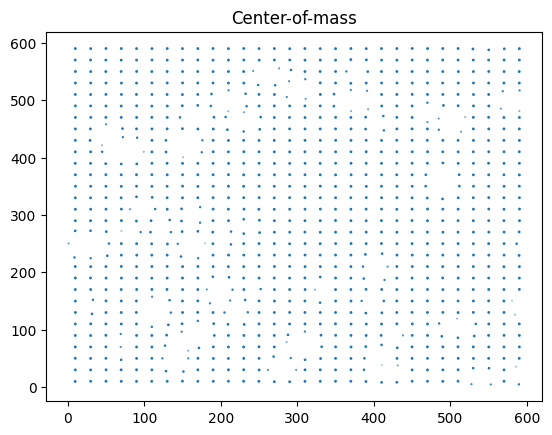
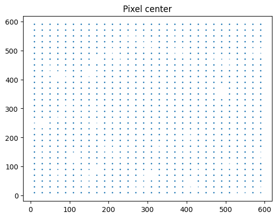
Reducing the catalog

Coarse-grains the tracers using a regular grid. This method is implicitly used when creating a hierarchical spatial hash, but one can also use it as a pre-processing step to reduce the number of tracers before inferring some summary statistic. Note that the reduce method does not place the catalog on a regular grid and does not return this as a 2d array, but instead either returns a suite of numpy nd arrays (default) or directly puts those into a corresponding catalog instance (for this set ret_inst=True).

We further allow for multiple options on where within the pixels to put the tracers:

• 0 –> Use center of mass. This is set as default

• 1 –> Do a random shift within the pixel. This does artificially add poisson noise to the couse-grained field which for estimates of large multipoles of the N PCF gives lower ringing effects

• 2 –> Use the pixel center

• 3 –> Use the position of the tracer with the largest weight

The following images showcase a few oth those choices and for visual purposes we set a fairly large pixelsize.

# Use center-of-mass. Size of points correspond to relative overdensity -- this is lower when the pixel intersects with a masked region
w_red, pos1_red, pos2_red, zbins_red, isinner_red, fields_red = shapecat.reduce(dpix=20., shuffle=0)
plt.scatter(pos1_red, pos2_red,s=w_red/np.mean(w_red))
plt.title('Center-of-mass')
plt.show()

# Same as above, but return as catalog instance. Check that both results are equivalent
red_cat = shapecat.reduce(dpix=20., shuffle=0, ret_inst=True)
print('Arrays agree?',np.array_equal(red_cat.pos1,pos1_red),np.array_equal(red_cat.pos2,pos2_red),np.array_equal(red_cat.weight,w_red))

# Use random shift within the pixel
w_red, pos1_red, pos2_red, zbins_red, isinner_red, fields_red = shapecat.reduce(dpix=20., shuffle=1)
plt.scatter(pos1_red, pos2_red,s=w_red/np.mean(w_red))
plt.title('Random shift within pixel')
plt.show()

# Use the pixel center
w_red, pos1_red, pos2_red, zbins_red, isinner_red, fields_red = shapecat.reduce(dpix=20., shuffle=2)
plt.scatter(pos1_red, pos2_red,s=w_red/np.mean(w_red))
plt.title('Pixel center')
plt.show()

Arrays agree? True True True

Constructing a (hierarchical) spatial hash

This is the main method orpheus uses for a quick range search operation. Here we just want to give some intuition of what this hash looks like – for the nitty gritty details please refer to the actual implementation. A single not worth making is that for a tomographic setup, we need to compute a separate hash for each tomographic bin.

In case a spatial hash is wanted for another application it can easily be constructed from the python layer using the multihash method. The main arguments that enter are the different pixel sizes of the hash (need to be multiples of two) as well as the shuffle parameter that we already encountered in the reduce method. The function then retuns a number of arrays from which a fast search can be constructed.

resos = [0.25,0.5,1.,2.,4.,8.]
hierarchical_hash = shapecat.multihash(dpixs=[0.25,0.5,1.,2.,4.,8.],shuffle=0)
ngals, pos1s, pos2s, weights, zbins, isinners, allfields, index_matchers, pixs_galind_bounds, pix_gals, dpixs1_true, dpixs2_true = hierarchical_hash

At first, let us have a quick look on what the hash achieved, i.e. how many galaxies are in the various reduced catalogs and how close the actual pixel size is the the target one (small discrepancies can happen to make the pixels evenly divide the extent of the survey footprint).

print('Galaxies per hash resolution: ',ngals)
print('True pixel sizes per resolution: ',dpixs1_true,dpixs2_true)

Galaxies per hash resolution:  [2750214, 2131981, 1138052, 324225, 81769, 20686, 5303]
True pixel sizes per resolution:  [0.2499999  0.4999998  0.9999996  1.99999921 3.99999842 7.99999683] [0.24999993 0.49999987 0.99999973 1.99999947 3.99999893 7.99999787]

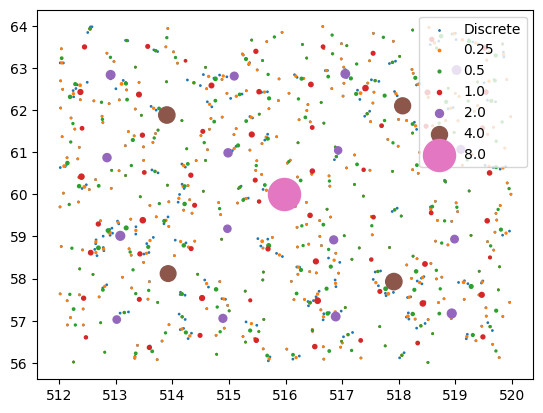
Now let us make a visualize the tracers that reside in each resolution of the catalog. For this we pick a single region that matches the size of the coarses cell-size in the hash. In the figure we further show the weight of each pixel as the size of each dot.

# The index of the spatial hash cell we are interested in
hash_target = 777

for elreso in range(7):
    if elreso==0:
        label='Discrete'
    else:
        label = resos[elreso-1]
    # Get the first and last indices of the galaxies within the pixel of the hash
    galind_bound_start = pixs_galind_bounds[elreso][index_matchers[elreso][hash_target]]
    galind_bound_end =  pixs_galind_bounds[elreso][index_matchers[elreso][hash_target]+1]
    # Retrieve those indices from the hierarchy of reduced catalogs
    galinds_elreso = pix_gals[elreso][galind_bound_start:galind_bound_end]
    plt.scatter(pos1s[elreso][galinds_elreso],pos2s[elreso][galinds_elreso],s=weights[elreso][galinds_elreso],label=label)
plt.legend(loc=1)
plt.show()

Building a mask

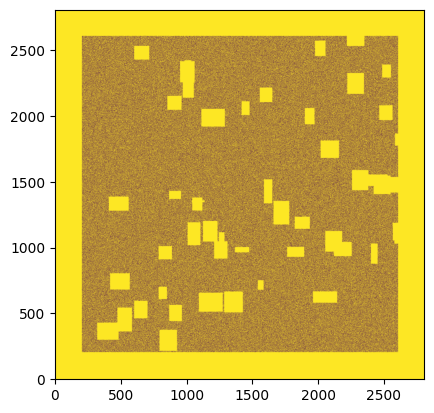
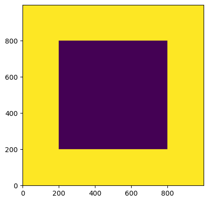
Methods such as the direct estimator require the specification of a survey mask based on the passed catalog. You can create such a mask using the create_mask method. Here we show three examples how this could be done.

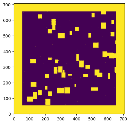
• Choose the default option –> This assumes no mask whatsoever and stores the mask values over the extent of the catalog. One can extend the maske over a larger range by setting the extend parameter.

• Reconstruct the mask from the observed tracers using method='Density' –> This first pixelizes the catalog and then assumes that empty pixels are masked.

• Reconstruct the mask from the observed tracers and additionally adjust the pixel size of the mask using the pixsize parameter –> Here you need to be careful to not choose the pixelsize too small as otherwise the density-based methods wrongly inferrs a mask in underdense regions. –> The default value is pixsize=1.0 which for most lensing applications gives a decent reconstruction if the units of the data are given in arcminutes.

shapecat.create_mask(extend=200)
plt.imshow(shapecat.mask.data,origin='lower')
print('Masked fraction: %.3f'%np.mean(shapecat.mask.data))
plt.show()


shapecat.create_mask(method='Density',extend=50)
plt.imshow(shapecat.mask.data,origin='lower')
print('Masked fraction: %.3f'%np.mean(shapecat.mask.data))
plt.show()

shapecat.create_mask(method='Density',pixsize=0.25,extend=50)
plt.imshow(shapecat.mask.data,origin='lower')
print('Masked fraction: %.3f'%np.mean(shapecat.mask.data))
plt.show()

Masked fraction: 0.640

Masked fraction: 0.353

Masked fraction: 0.730