Computing galaxy-galaxy-galaxy lensing statistics

In this notebooks we compute the galaxy-galaxy-galaxy lensing (G3L) shear correlation functions on a mock catalog and transform them to the third-order aperture statistics.

from astropy.table import Table
import numpy as np
from matplotlib import pyplot as plt

import orpheus

Initialize the catalog instances

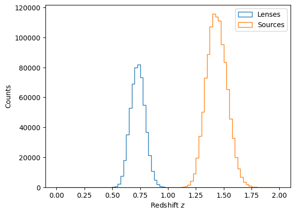
For this exercise we use a simplistic mock catalog built from the Takahasi simulation suite that traces two tomographic bins in a Euclid-like setup for the \(n(z)\) and uses a linear galaxy bias.

As we are dealing with two separate catalogs, we need to initialize a ScalarTracerCatalog instance for the lenses and a SpinTracerCatalog (with spin=2) for the sources.

catname = "data_g3l.npz"

mock = np.load(catname)

plt.hist(mock['z_lens_true'],bins=np.linspace(0,2,81),histtype='step',lw=3,label='Lenses')
plt.hist(mock['z_source_true'],bins=np.linspace(0,2,81),histtype='step',lw=3,label='Sources')
plt.xlabel(r'Redshift $z$')
plt.ylabel('Counts')
plt.legend()
plt.show()

sources = orpheus.SpinTracerCatalog(spin=2,
                                    pos1=mock["x_source"],
                                    pos2=mock["y_source"],
                                    tracer_1=mock["gam1_source"],
                                    tracer_2=mock["gam2_source"],
                                    weight=None, zbins=None)
lenses = orpheus.ScalarTracerCatalog(pos1=mock["x_lens"],
                                     pos2=mock["y_lens"],
                                     tracer=np.ones_like(mock["x_lens"]),
                                     weight=None, zbins=None)

print("Number of source galaxies:%i --> effective nbar: %.3f/arcmin^2 on %.2f deg^2"%(
    sources.ngal, sources.ngal/(sources.len1*sources.len2), sources.len1*sources.len2/3600.))
print("Number of lens galaxies:%i --> effective nbar: %.3f/arcmin^2 on %.2f deg^2"%(
    lenses.ngal, lenses.ngal/(lenses.len1*lenses.len2), lenses.len1*lenses.len2/3600.))

Number of source galaxies:1098203 --> effective nbar: 2.848/arcmin^2 on 107.10 deg^2
Number of lens galaxies:551207 --> effective nbar: 1.431/arcmin^2 on 107.02 deg^2

Computation of the shear-lens-lens correlation function

For computing the shear-lens-lens correlation function we need to invoke the GNNCorrelation class. In principle, it is only required to define a binning for the 3pcf (given by the range of the bins and the number of bins).

Notes

• Instead of the number of bins you can also specify the logarithmic bin-width binsize. However, the final value of binsize might differ slightly from the provided one as we fix the values for the binning range and then choose the largest possible value of binsize that is smaller or equal to the input value for binsize.

• If no further parameters are passed, the default setup chooses the some accelerations of the discrete multipole estimator renders fairly accurate results for the 3pcf itself and percent-level accuracy for the third-order aperture statistics. In case you want a different setup than the default results you can change the parameters of the parent BinnedNPCF class.

min_sep = 0.25
max_sep = 150.
binsize = 0.1
nbinsphi = 256
method = "DoubleTree"
resoshift_leafs=-2
nthreads = 48

gnn = orpheus.GNNCorrelation(min_sep=min_sep,
                                 max_sep=max_sep,
                                 binsize=binsize,
                                 nbinsphi=nbinsphi,
                                 method=method,
                                 resoshift_leafs=resoshift_leafs,
                                 nthreads=nthreads,verbosity=2)

%%time
gnn.process(sources, lenses)

Done 99.95 per centCPU times: user 35min 8s, sys: 3.06 s, total: 35min 11s
Wall time: 49.6 s

Once processed, the instance of GNNCorrelation contains the multipole components of the shear-lens-lens correlators \(\Upsilon^{'}_{\tilde{\mathcal{G}},n}\), as well as their nonrmalizations \(\mathcal{W}_n\) in their multipole basis. If required, we can use the multiples2npcf method to transform the to the real-space basis, in which they become the more well-known shear-lens-lens correlation function \(\tilde{G}\) introduced in Schneider & Watts 2005.

%%time
gnn.multipoles2npcf()

CPU times: user 528 ms, sys: 8 ms, total: 536 ms
Wall time: 534 ms

Computation of the aperture statistics

The integral transormation between the shear-lens-lens 3PCF and their third-order aperture statistics can be done by calling the GNNNCorrelation.computeNNM method.

Notes

• In case you are only interested in obtaining the third-order aperture statistics, you can also directly call this method right after processing the shape catalog.

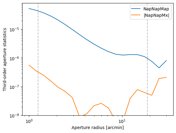
• One should only trust the third-order aperture statistics for radii \(R\in[\alpha\,\theta_{\rm min}, \beta\,\theta_{\rm max}]\), where \(\alpha\approx 5\) and \(\beta \approx 0.125\). In the plot below this range is indicated by the dashed vertical lines.

• Furthermore, the binning should be sufficiently fine, i.e. the value of the GNNCorrelation.binsize attribute should be less than 0.1 for an accuracy of about one per cent.

%%time
radii_ap = np.geomspace(1.,30.,20)
NNM = gnn.computeNNM(radii_ap)

CPU times: user 9.21 s, sys: 753 ms, total: 9.96 s
Wall time: 3.95 s

plt.loglog(radii_ap, NNM[0,0].real, label="NapNapMap")
plt.loglog(radii_ap, np.abs(NNM[0,0].imag), label="|NapNapMx|")
plt.axvline(x=5*gnn.min_sep, color="grey",alpha=0.5,ls="--")
plt.axvline(x=0.125*gnn.max_sep, color="grey",alpha=0.5,ls="--")
plt.xlabel("Aperture radius [arcmin]")
plt.ylabel("Third-order aperture statistics")
plt.legend(loc="upper right")
plt.ylim(1e-8,None)

(1e-08, 8.290079304338584e-05)

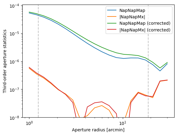
Accounting for the angular clustering correlation function

The estimator for the 3pcf described above is biased as the lenses are inherently clustered which implies that we perform the area-averaging of the source-lens-lens pairs in a non-uniform fashion (see Simon et al. 2008 for further details). To counter this effect we need to modify the estimator and reweight the nominator by the same factor.

We give the option to apply this correction within the multipoles2npcf method when making use of the optional xi parameter. The data type of xi is defined to be a list of two elements: * The zeroth element are the radial bin centers at which the clustering 2pcf is evaluated * The first element is the clustering 2pcf for all tomographic (lens) bin combinations

This general way to pass the clustering 2pcf allows for both, a theoretical and a measurement-based model. For our example we make use of the measured clustering 2pcf from the NN_tutorial notebook.

Note: Our prescription slightly differs from the original one introduced inSimon et al. 2008as the multiple-decomposition of the triplet counts do not contain information about the shape of each individual triangle – only its mean shape per bin is known. Given the smooth shape of the clustering correlation function, for a sufficiently fine binning in radial and angular scales the two prescriptions should converge towards each other.

# Load in the data that we stored in NN_tutorial.ipynb
dat_nn = np.load("nncorr.npz")

# Define xi.
# As in NN_tutorial.ipynb we computed the 2pcf for all tomographic bin combinations we need to select the
# lens-lens one. This is the zeroth index. The double brackets are needed to make sure the shape matches
# the orpheus convention for which xi[1].shape == (nzlens*nzlens, nbinsr)
xi_corr = [dat_nn['bin_centers_mean'], dat_nn['xi'][[0]]]

We now repeat the computation of the conversion between multipole-space and real-space and the convert to the aperture statistics.

%%time
gnn.multipoles2npcf(xi=xi_corr)
NNM_wcorr = gnn.computeNNM(radii_ap)

CPU times: user 6.37 s, sys: 269 ms, total: 6.64 s
Wall time: 771 ms

When comparing both results we see that the clustering-induced correction boosts the E-mode aperture statistics while it does not siginficantly affect the B-Mode.

plt.loglog(radii_ap, NNM[0,0].real, label="NapNapMap")
plt.loglog(radii_ap, np.abs(NNM[0,0].imag), label="|NapNapMx|")
plt.loglog(radii_ap, NNM_wcorr[0,0].real, label="NapNapMap (corrected)")
plt.loglog(radii_ap, np.abs(NNM_wcorr[0,0].imag), label="|NapNapMx| (corrected)")
plt.axvline(x=5*gnn.min_sep, color="grey",alpha=0.5,ls="--")
plt.axvline(x=0.125*gnn.max_sep, color="grey",alpha=0.5,ls="--")
plt.xlabel("Aperture radius [arcmin]")
plt.ylabel("Third-order aperture statistics")
plt.legend(loc="upper right")
plt.ylim(1e-8,None)

(1e-08, 0.00010657315314739559)

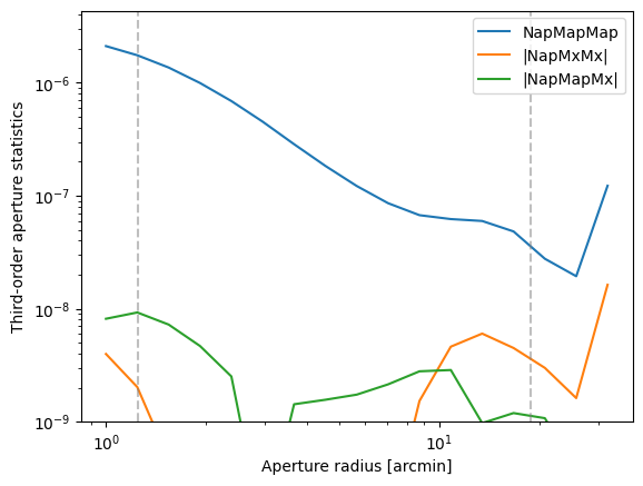
Computation of the lens-shear-shear correlation function

Let us now repeat the same procedure for the NGG correlation – the stragegy is practically the same as for GNN. However, we note that due to the multipole structure of \(\tilde{G}_+\) we need to choose a fairly large value for rmin_pixsize as otherwise the tree-based approximations can produce an artificial \(\langle N_{ap}M_{\times}^2 \rangle\) mode.

We further note that the different components of the NGG correlator are ordered as :math:`[ tilde{G}_-, tilde{G}_+ ]` , which is different to the usual conventions, but matches ``orpheus``’ conventions to always start with a correlator in which not polar field is complex conjugated.

min_sep = 0.25
max_sep = 150.
binsize = 0.1
nbinsphi = 256
tree_resos = [0.,1.,2.]
rmin_pixsize=40
method = "DoubleTree"
nthreads = 48

ngg = orpheus.NGGCorrelation(min_sep=min_sep,
                             max_sep=max_sep,
                             binsize=binsize,
                             nbinsphi=nbinsphi,
                             method=method,
                             rmin_pixsize=rmin_pixsize,
                             tree_resos=tree_resos,
                             nthreads=nthreads,verbosity=2)

%%time
ngg.process(sources, lenses)

.........|.........|.........|.........|.........|.........|.........|.........|.........|.........|CPU times: user 1h 37min 57s, sys: 6.03 s, total: 1h 38min 3s
Wall time: 2min 3s

%%time
ngg.multipoles2npcf()

CPU times: user 680 ms, sys: 7 ms, total: 687 ms
Wall time: 684 ms

%%time
radii_ap = np.geomspace(1.,32.,17)
NMM = ngg.computeNMM(radii_ap)

CPU times: user 11.9 s, sys: 8.1 s, total: 20 s
Wall time: 3.89 s

plt.loglog(radii_ap, NMM[0,0], label="NapMapMap")
plt.loglog(radii_ap, np.abs(NMM[1,0]), label="|NapMxMx|")
plt.loglog(radii_ap, np.abs(NMM[2,0]), label="|NapMapMx|")
plt.axvline(x=5*ngg.min_sep, color="grey",alpha=0.5,ls="--")
plt.axvline(x=0.125*ngg.max_sep, color="grey",alpha=0.5,ls="--")
plt.xlabel("Aperture radius [arcmin]")
plt.ylabel("Third-order aperture statistics")
plt.legend(loc="upper right")
plt.ylim(1e-9,None)

/users/lporth/anaconda3/envs/orpheus_devel/lib/python3.12/site-packages/matplotlib/cbook.py:1709: ComplexWarning: Casting complex values to real discards the imaginary part
  return math.isfinite(val)
/users/lporth/anaconda3/envs/orpheus_devel/lib/python3.12/site-packages/matplotlib/cbook.py:1345: ComplexWarning: Casting complex values to real discards the imaginary part
  return np.asarray(x, float)

(1e-09, 4.355715096918785e-06)