Computing higher-order aperture mass measures using the direct estimator

In this notebook we compute the equal-scale higher-order aperture mass moments on a shape catalog using the direct estimator introduced in Schneider+ (1998) and extended in Porth & Smith (2022).

from astropy.table import Table
import numpy as np
from matplotlib import pyplot as plt

import orpheus

## Obtaining a realistic mock shape catalog

We will run this notebook using a mocks shape catalog from the SLICS ensemble. First, let us download this catalog and read in its contents and then split it in three tomographic bins.

Note: If you want to run the notebook yourself, you need to update the savepath_SLICS variable.

catname = "GalCatalog_LOS1.fits"
path_to_SLICS = "http://cuillin.roe.ac.uk/~jharno/SLICS/MockProducts/KiDS450/" + catname
savepath_SLICS = "/vol/euclidraid4/data/lporth/HigherOrderLensing/Mocks/SLICS_KiDS450/"
nbinsz = 3

#!wget {path_to_SLICS} -P {savepath_SLICS}

slicscat = Table.read(savepath_SLICS + catname)
print(slicscat.keys())

['x_arcmin', 'y_arcmin', 'z_spectroscopic', 'z_photometric', 'shear1', 'shear2', 'eps_obs1', 'eps_obs2']

WARNING: UnitsWarning: 'UNKNOWN' did not parse as fits unit: At col 0, Unit 'UNKNOWN' not supported by the FITS standard.  If this is meant to be a custom unit, define it with 'u.def_unit'. To have it recognized inside a file reader or other code, enable it with 'u.add_enabled_units'. For details, see https://docs.astropy.org/en/latest/units/combining_and_defining.html [astropy.units.core]
WARNING: UnitsWarning: 'UNKNOWN' did not parse as fits unit: At col 0, Unit 'UNKNOWN' not supported by the FITS standard.  If this is meant to be a custom unit, define it with 'u.def_unit'. To have it recognized inside a file reader or other code, enable it with 'u.add_enabled_units'. For details, see https://docs.astropy.org/en/latest/units/combining_and_defining.html [astropy.units.core]

# Split in three tomographic bins
slicscat = Table.read(savepath_SLICS+"GalCatalog_LOS1.fits")
zbins = (slicscat['z_spectroscopic']/0.5).astype(int).data
zbins[zbins>(nbinsz-1)] = nbinsz-1

WARNING: UnitsWarning: 'UNKNOWN' did not parse as fits unit: At col 0, Unit 'UNKNOWN' not supported by the FITS standard.  If this is meant to be a custom unit, define it with 'u.def_unit'. To have it recognized inside a file reader or other code, enable it with 'u.add_enabled_units'. For details, see https://docs.astropy.org/en/latest/units/combining_and_defining.html [astropy.units.core]
WARNING: UnitsWarning: 'UNKNOWN' did not parse as fits unit: At col 0, Unit 'UNKNOWN' not supported by the FITS standard.  If this is meant to be a custom unit, define it with 'u.def_unit'. To have it recognized inside a file reader or other code, enable it with 'u.add_enabled_units'. For details, see https://docs.astropy.org/en/latest/units/combining_and_defining.html [astropy.units.core]

Initialize the catalog instance

As we are dealing with an ellipticity catalog, we need to use the SpinTracerCatalog class and set the value of spin to two.

shapecat = orpheus.SpinTracerCatalog(spin=2,
                                     pos1=slicscat["x_arcmin"],
                                     pos2=slicscat["y_arcmin"],
                                     zbins=zbins,
                                     tracer_1=slicscat["shear1"],
                                     tracer_2=slicscat["shear2"])

print("Number of galaxies:%i --> effective nbar: %.3f/arcmin^2 on %.2f deg^2"%(
    shapecat.ngal, shapecat.ngal/(shapecat.len1*shapecat.len2), shapecat.len1*shapecat.len2/3600.))

Number of galaxies:3070801 --> effective nbar: 8.530/arcmin^2 on 100.00 deg^2

As the direct estimator is formally only defined on survey fields without holes or boundaries, we need to construct a mask that checks in which regions this assumption is not fulfilled. For our idealised example we simply use the default setup that is defined as the rectangular bounding box of the shape catalog as the survey mask.

shapecat.create_mask()

## Computation of the equal-scale aperture mass statistics (non-tomographic)

For utilising the direct estimator for aperture mass statistics we need to invoke the Direct_MapnEqual class which derives from the more general DirectEstimator class.

Notes

• At the moment we only include a logarithmic binning of aperture radii. This can either be specified by the number of bins (nbinsr) or the logarithmic bin size (binsize)

• At the moment we have not implemented tree-based catalog reductions that are used for the NPCF computation – setting the corresponding parameters in the DirectEstimator does not have an effect.

• The computation of the aperture statistics is done recusively, that is by specifying order_max one retrieves all aperture statistics up to order_max.

• For assessing the impact of a nontrivial survey mask in a several run we simulanously compute the aperture statistics for a variety of coverage cuts that only include apertures that are covered by at most a fraction frac_cov. The location and number of those cuts is set by the frac_covs attribute.

• There are multiple parameters that can be set to tweak the estimator to be optimal for a specific survey setup. The default values are chosen such that the low-order statistics are expected to converge for stage-III-like surveys. The accuracy can adapted by changing the accuracies attribute – note that the runtime increases quadratically with this attribute.

orpheus.Direct_MapnEqual.__init__

<function orpheus.direct.Direct_MapnEqual.__init__(self, order_max, Rmin, Rmax, field='polar', filter_form='C02', ap_weights='InvShot', **kwargs)>

orpheus.DirectEstimator.__init__

<function orpheus.direct.DirectEstimator.__init__(self, Rmin, Rmax, nbinsr=None, binsize=None, aperture_centers='grid', accuracies=2.0, frac_covs=[0.0, 0.1, 0.3, 0.5, 1.0], dpix_hash=1.0, weight_outer=1.0, weight_inpainted=0.0, method='Discrete', multicountcorr=True, shuffle_pix=1, tree_resos=[0, 0.25, 0.5, 1.0, 2.0], tree_redges=None, rmin_pixsize=20, resoshift_leafs=0, minresoind_leaf=None, maxresoind_leaf=None, nthreads=16)>

Rmin = 1.
Rmax = 32.
nbinsr = 12
frac_covs=[0.0, 0.1, 0.3, 0.5, 1.0]
order_max = 6
nthreads = 48

direct = orpheus.Direct_MapnEqual(order_max=order_max, Rmin=Rmin, Rmax=Rmax, nbinsr=nbinsr, nthreads=nthreads)

When running the direct estimator we can choose whether to use the tomographic information in the shape catalog

%%time
mapn, mapn_weights = direct.process(shapecat,dotomo=False)

/users/lporth/anaconda3/envs/orpheus_devel/lib/python3.12/site-packages/orpheus/catalog.py:738: RuntimeWarning: invalid value encountered in divide
  projectedfields[:,1:] = np.nan_to_num(projectedfields[:,1:]/projectedfields[:,0])

Done 12/12 aperture radiiCPU times: user 13min 58s, sys: 1.43 s, total: 13min 59s
Wall time: 23.6 s

Once the catalog is processed, the method returns the aperture statistics as well as the cumulative aperture weights of the shape catalog. The latter is required when combining measurements from multiple small patches of a large catalog by using a weighted average.

The shape of both outputs is equal and given as (nbinsr, nfrac_cov, nzcombis) where nzcombis collects all possible combinations of redshift bins up to order_max.

mapn.shape

(12, 5, 6)

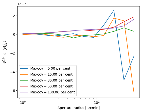
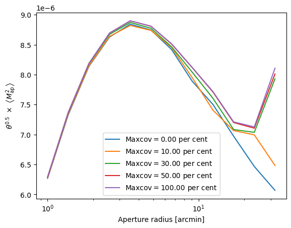
for order in range(direct.order_max):
    for covcut in range(direct.nfrac_covs):
        plt.semilogx(direct.radii, direct.radii**(.5*order)*mapn[:,covcut,order],label=r'$\rm{Max cov}=%.2f$ per cent'%(100*direct.frac_covs[covcut]))
        plt.xlabel('Aperture radius [arcmin]')
        plt.ylabel(r'$\theta^{%.1f} \ \times \ \left\langle M_{\rm ap}^%i\right\rangle$'%((0.5*order),order+1))
        plt.legend()
    plt.show()

Computation of the equal-scale aperture mass statistics (tomographic)

Now let us repeat the same calculation with tomography

%%time
mapn, mapn_weights = direct.process(shapecat,dotomo=True)

Done 12/12 aperture radiiCPU times: user 14min 38s, sys: 567 ms, total: 14min 39s
Wall time: 25.8 s

Looking at the shape we see that the number of tomographic bin combinations quickly blows up.

mapn.shape

(12, 5, 83)

For being able to readily access a specific tomographic bin combination one can use the genzcombi method which gives the correct index for a tomographic bin combination \((z_1,\cdots,z_k)\). Note that we only allocate combinations with \(z_i \leq z_{i+1}\).

direct.genzcombi([0,1,1,2])

26

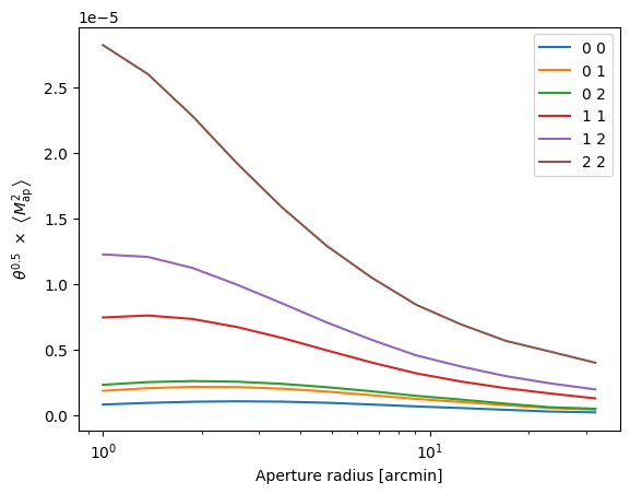
elcov = 0
# Order = 2
for z1 in range(shapecat.nbinsz):
    for z2 in range(z1,shapecat.nbinsz):
        zcombi = direct.genzcombi([z1,z2])
        plt.semilogx(direct.radii, mapn[:,elcov,direct.genzcombi([z1,z2])],label='%i %i'%(z1,z2))
plt.xlabel('Aperture radius [arcmin]')
plt.ylabel(r'$\theta^{%.1f} \ \times \ \left\langle M_{\rm ap}^%i\right\rangle$'%((0.5),2))
plt.legend()
plt.show()

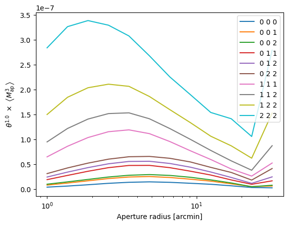
# Order = 3
for z1 in range(shapecat.nbinsz):
    for z2 in range(z1,shapecat.nbinsz):
        for z3 in range(z2,shapecat.nbinsz):
            zcombi = direct.genzcombi([z1,z2,z3])
            plt.semilogx(direct.radii, direct.radii*mapn[:,elcov,direct.genzcombi([z1,z2,z3])],label='%i %i %i'%(z1,z2,z3))
plt.xlabel('Aperture radius [arcmin]')
plt.ylabel(r'$\theta^{%.1f} \ \times \ \left\langle M_{\rm ap}^%i\right\rangle$'%((1),3))
plt.legend()
plt.show()

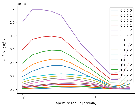
# Order = 4
for z1 in range(shapecat.nbinsz):
    for z2 in range(z1,shapecat.nbinsz):
        for z3 in range(z2,shapecat.nbinsz):
            for z4 in range(z3,shapecat.nbinsz):
                _full = mapn[:,elcov,direct.genzcombi([z1,z2,z3,z4])]
                _disc = (mapn[:,elcov,direct.genzcombi([z1,z2])] * mapn[:,elcov,direct.genzcombi([z3,z4])] +
                        mapn[:,elcov,direct.genzcombi([z1,z3])] * mapn[:,elcov,direct.genzcombi([z2,z4])] +
                        mapn[:,elcov,direct.genzcombi([z1,z4])] * mapn[:,elcov,direct.genzcombi([z2,z3])])
                plt.semilogx(direct.radii, direct.radii**1.5*(_full-_disc),label='%i %i %i %i'%(z1,z2,z3,z4))
plt.xlabel('Aperture radius [arcmin]')
plt.ylabel(r'$\theta^{%.1f} \ \times \ \left\langle M_{\rm ap}^%i\right\rangle$'%((1.5),4))
plt.legend()
plt.show()

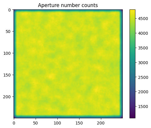
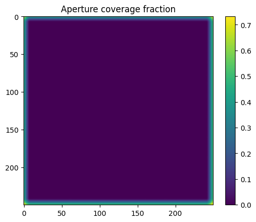
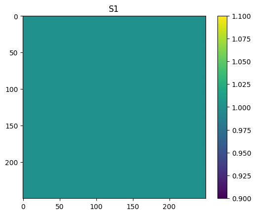
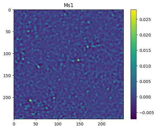
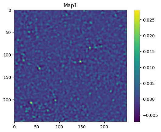
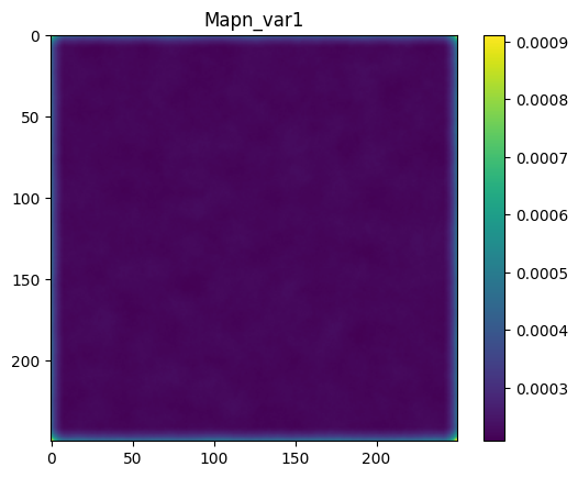
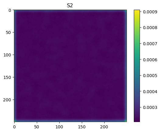
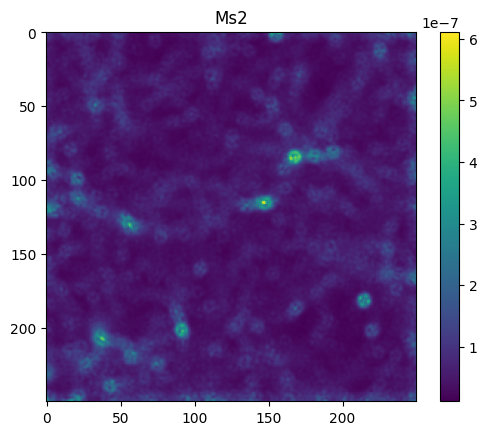
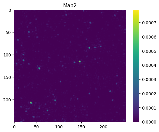
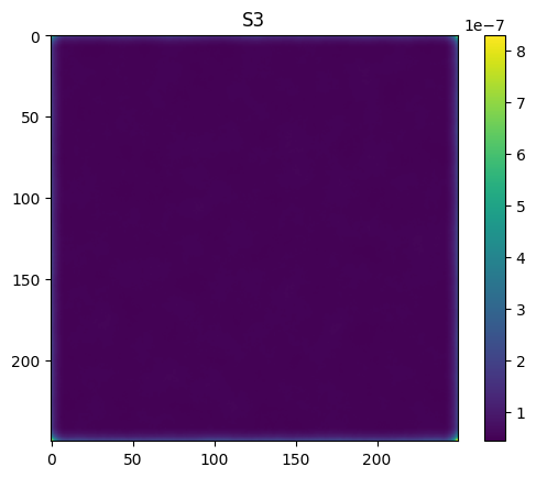
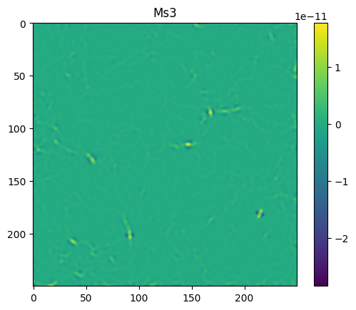
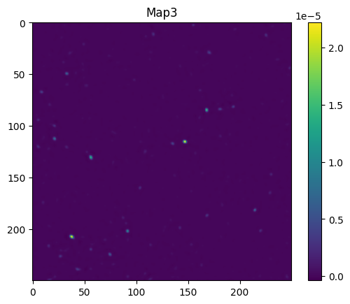
## Computing aperture mass maps

For a more visual inspection of the ingredients going into the computation of the direct estimator we also provide a method to compute the aperture mass map from a shape catalog. We use the same basis that was introduced in Porth & Smith 2021 (see Eq 22, 23 for the Sn and Msn and Eq 43 for the inverse-variance weights).

# Index of aperture radius to consider
indR = 5
print(direct.radii[indR])

4.832357777617789

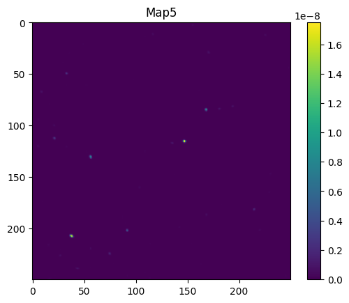
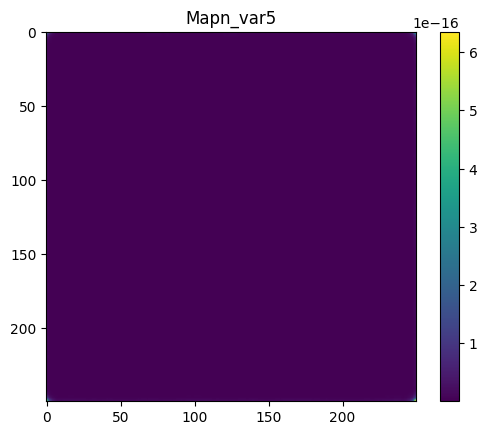
counts, covs, Msn, Sn, Mapn, Mapn_var = direct.getmap(indR, shapecat, dotomo=True)

elbinz = 1
plt.imshow(counts[elbinz,0])
plt.colorbar()
plt.title('Aperture number counts')
plt.show()

plt.imshow(covs[0])
plt.colorbar()
plt.title('Aperture coverage fraction')
plt.show()

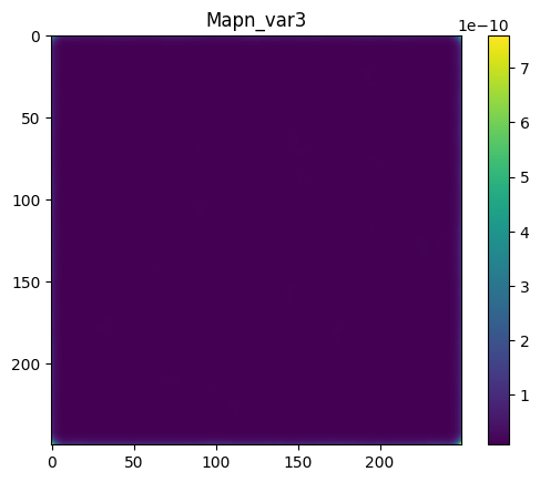
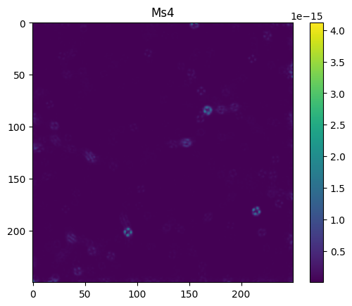
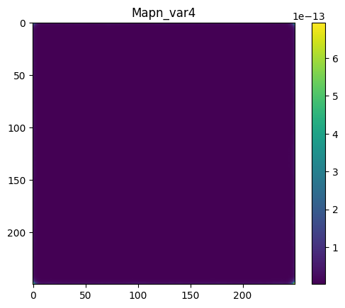
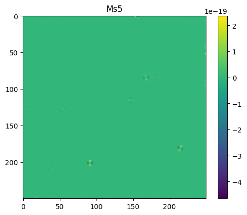
for order in range(direct.order_max):
    plt.imshow(Sn[elbinz,order])
    plt.colorbar()
    plt.title('S%i'%(order+1))
    plt.show()

    plt.imshow(Msn[elbinz,order])
    plt.colorbar()
    plt.title('Ms%i'%(order+1))
    plt.show()

    plt.imshow(Mapn[elbinz,order])
    plt.colorbar()
    plt.title('Map%i'%(order+1))
    plt.show()

    plt.imshow(np.abs(Mapn_var[elbinz,order]))
    plt.colorbar()
    plt.title('Mapn_var%i'%(order+1))
    plt.show()