Computing third-order shear statistics on a shape catalog

In this notebooks we compute the third-order shear correlation functions on a realistic shape catalog and transform them to the third-order aperture statistics.

from astropy.table import Table
from itertools import combinations_with_replacement
import numpy as np
from matplotlib import pyplot as plt

import orpheus

Obtaining a realistic mock shape catalog

We will run this notebook using a mocks shape catalog from the SLICS ensemble. First, let us download this catalog and read in its contents.

Note: If you want to run the notebook yourself, you need to update the savepath_SLICS variable.

catname = "GalCatalog_LOS1.fits"
path_to_SLICS = "http://cuillin.roe.ac.uk/~jharno/SLICS/MockProducts/KiDS450/" + catname
savepath_SLICS = "/vol/euclidraid4/data/lporth/HigherOrderLensing/Mocks/SLICS_KiDS450/"

#!wget {path_to_SLICS} -P {savepath_SLICS}

slicscat = Table.read(savepath_SLICS + catname)
print(slicscat.keys())

['x_arcmin', 'y_arcmin', 'z_spectroscopic', 'z_photometric', 'shear1', 'shear2', 'eps_obs1', 'eps_obs2']

WARNING: UnitsWarning: 'UNKNOWN' did not parse as fits unit: At col 0, Unit 'UNKNOWN' not supported by the FITS standard.  If this is meant to be a custom unit, define it with 'u.def_unit'. To have it recognized inside a file reader or other code, enable it with 'u.add_enabled_units'. For details, see https://docs.astropy.org/en/latest/units/combining_and_defining.html [astropy.units.core]
WARNING: UnitsWarning: 'UNKNOWN' did not parse as fits unit: At col 0, Unit 'UNKNOWN' not supported by the FITS standard.  If this is meant to be a custom unit, define it with 'u.def_unit'. To have it recognized inside a file reader or other code, enable it with 'u.add_enabled_units'. For details, see https://docs.astropy.org/en/latest/units/combining_and_defining.html [astropy.units.core]

Initialize the catalog instance

As we are dealing with an ellipticity catalog, we need to use the SpinTracerCatalog class and set the value of spin to two.

shapecat = orpheus.SpinTracerCatalog(spin=2,
                                     pos1=slicscat["x_arcmin"],
                                     pos2=slicscat["y_arcmin"],
                                     tracer_1=slicscat["shear1"],
                                     tracer_2=slicscat["shear2"])

print("Number of galaxies:%i --> effective nbar: %.3f/arcmin^2 on %.2f deg^2"%(
    shapecat.ngal, shapecat.ngal/(shapecat.len1*shapecat.len2), shapecat.len1*shapecat.len2/3600.))

Number of galaxies:3070801 --> effective nbar: 8.530/arcmin^2 on 100.00 deg^2

Computation of the shear 3pcf

For computing the natural components of the third-order shear correlation functions we need to invoke the GGGCorrelation class. In principle, it is only required to define a binning for the 3pcf (given my the range of the bins and the number of bins).

Notes

• Instead of the number of bins you can also specify the logarithmic bin-width binsize. However, the final value of binsize might differ slightly from the provided one as we fix the values for the binning range and then choose the largest possible value of binsize that is smaller or equal to the input value for binsize.

• If no further parameters are passed, the default setup chooses the some accelerations of the discrete multipole estimator renders fairly accurate results for the 3pcf itself and percent-level accuracy for the third-order aperture statistics. In case you want a different setup than the default results you can change the parameters of the parent BinnedNPCF class.

orpheus.GGGCorrelation.__init__

<function orpheus.npcf_third.GGGCorrelation.__init__(self, n_cfs, min_sep, max_sep, **kwargs)>

orpheus.BinnedNPCF.__init__

<function orpheus.npcf_base.BinnedNPCF.__init__(self, order, spins, n_cfs, min_sep, max_sep, nbinsr=None, binsize=None, nbinsphi=100, nmaxs=30, method='DoubleTree', multicountcorr=True, shuffle_pix=0, tree_resos=[0, 0.25, 0.5, 1.0, 2.0], tree_redges=None, rmin_pixsize=20, resoshift_leafs=0, minresoind_leaf=None, maxresoind_leaf=None, methods_avail=['Discrete', 'Tree', 'BaseTree', 'DoubleTree'], verbosity=0, nthreads=16)>

min_sep = 0.5
max_sep = 150.
binsize = 0.1
nthreads=48

threepcf = orpheus.GGGCorrelation(n_cfs=4,
                                  min_sep=min_sep, max_sep=max_sep,binsize=binsize,
                                  nthreads=nthreads, verbosity=2)

%%time
threepcf.process(shapecat)

.........|.........|.........|.........|.........|.........|.........|.........|.........|.........|
CPU times: user 2h 1min 45s, sys: 7 s, total: 2h 1min 52s
Wall time: 2min 36s

Once processed, the instance of GGGCorrelation contains the multipole components of the third-order shear correlators \(\Upsilon_{\mu,n}\), as well as their nonrmalizations \(\mathcal{N}_n\) in their multipole basis. If required, we can use the multiples2npcf method to transform the to the real-space basis, in which they become the more well-known natural components \(\Gamma_{\mu}\) of the shear 3PCF (Schneider 2003).

%%time
threepcf.multipoles2npcf()

CPU times: user 939 ms, sys: 6.03 ms, total: 945 ms
Wall time: 27.7 ms

Unless otherwise specified, the projection of the shear is not altered - hence it is given in the projection favoured by the multipole estimator, which in orpheus is dubbed the X-projection. To transform it the the centroid projection we can use the projectnpcf methods. The current projection can always be accessed by the projection attribute.

%%time
print("Current 3PCF projection: %s"%threepcf.projection)
threepcf.projectnpcf("Centroid")
print("Current 3PCF projection: %s"%threepcf.projection)

Current 3PCF projection: Centroid
Current 3PCF projection: Centroid
CPU times: user 0 ns, sys: 247 µs, total: 247 µs
Wall time: 247 µs

Computation of the aperture mass

The integral transormation between the shear 3PCF and the third-order aperture statistics can be done by calling the GGGCorrelation.computeMap3 method. We can trigger the evauluation of the unequal scale statistics by setting do_multiscale=True, otherwise the equal-scale statistics are computed.

Notes

• In case you are only interested in obtaining the third-order aperture statistics, you can also directly call this method right after processing the shape catalog.

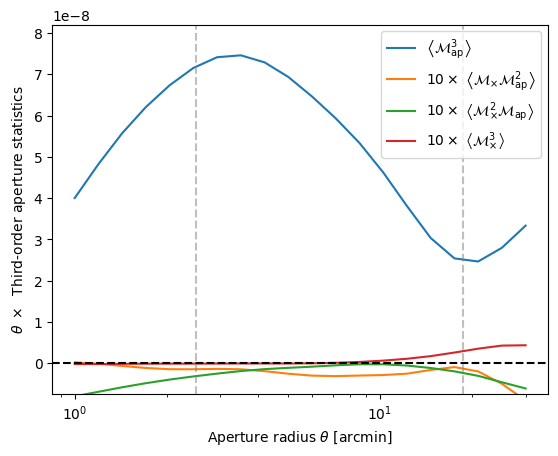
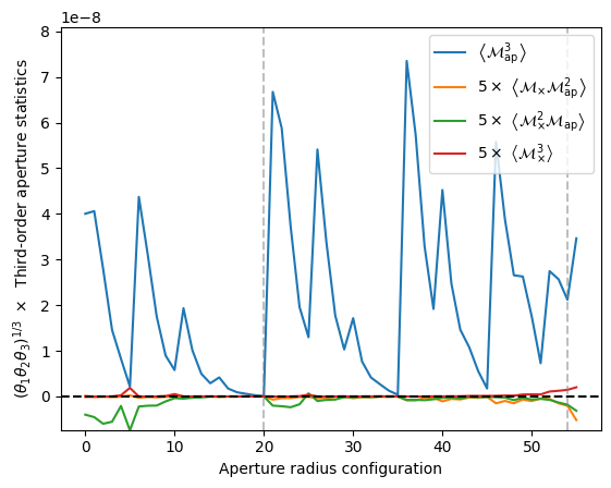
• One should only trust the third-order aperture statistics for radii \(R\in[\alpha\,\theta_{\rm min}, \beta\,\theta_{\rm max}]\), where \(\alpha\approx 5\) and \(\beta \approx 0.125\). In the plot below this range is indicated by the dashed vertical lines.

• Furthermore, the binning should be sufficiently fine, i.e. the value of the GGGCorrelation.binsize attribute should be less than 0.1 for an accuracy of about one per cent.

mapradii = np.geomspace(1,30,20)
mapradii_multi = np.geomspace(1,32,6)

%%time
map3 = threepcf.computeMap3(mapradii)

CPU times: user 4.72 s, sys: 144 ms, total: 4.87 s
Wall time: 4.99 s

%%time
_map3_multi = threepcf.computeMap3(mapradii_multi,do_multiscale=True)
map3_multi = orpheus.symmetrize_map3_multiscale(_map3_multi) # Symmetrize the output (Map3 is symmetric in the three aperture radii)

CPU times: user 20.6 s, sys: 37 ms, total: 20.7 s
Wall time: 20.7 s

scaleB = 10 # Rescale the B-modes for better visualization
scaleP = 10 # Rescale the parity-violating-modes for better visualization
plt.semilogx(mapradii,mapradii*map3[0,0].real, label=r"$\left\langle \mathcal{M}_{\rm ap}^3\right\rangle$")
plt.semilogx(mapradii,mapradii*scaleP*np.mean(map3[[1,2,3],0].real,axis=0), label=r"$ %i \times \ \left\langle  \mathcal{M}_{\times} \mathcal{M}_{\rm ap}^2\right\rangle$"%scaleP)
plt.semilogx(mapradii,mapradii*scaleB*np.mean(map3[[4,5,6],0].real,axis=0), label=r"$ %i \times \ \left\langle  \mathcal{M}_{\times}^2 \mathcal{M}_{\rm ap}\right\rangle$"%scaleB)
plt.semilogx(mapradii,mapradii*scaleP*map3[7,0].real, label=r"$ %i \times \ \left\langle  \mathcal{M}_{\times}^3 \right\rangle$"%scaleP)
plt.axvline(x=5*threepcf.min_sep, color="grey",alpha=0.5,ls="--")
plt.axvline(x=0.125*threepcf.max_sep, color="grey",alpha=0.5,ls="--")
plt.axhline(y=0,color="black",ls="--")
plt.xlabel(r"Aperture radius $\theta$ [arcmin]")
plt.ylabel(r"$\theta \ \times \ $ Third-order aperture statistics")
plt.ylim(-.1*np.max(mapradii*map3[0,0].real),1.1*np.max(mapradii*map3[0,0].real))
plt.legend(loc='upper right')
plt.show()


scaleB = 5 # Rescale the B-modes for better visualization
scaleP = 5 # Rescale the parity-violating-modes for better visualization
norm = np.array([np.prod(mapradii_multi[list(c)]) for c in combinations_with_replacement(range(len(mapradii_multi)), 3)])**(1./3.) # Our normalization, (theta1*theta2*theta3)^(1/3)
plt.plot(np.arange(len(norm)),norm*map3_multi[0,0].real, label=r"$\left\langle \mathcal{M}_{\rm ap}^3\right\rangle$")
plt.plot(np.arange(len(norm)),norm*scaleP*np.mean(map3_multi[[1,2,3],0].real,axis=0), label=r"$ %i \times \ \left\langle  \mathcal{M}_{\times} \mathcal{M}_{\rm ap}^2\right\rangle$"%scaleP)
plt.plot(np.arange(len(norm)),norm*scaleB*np.mean(map3_multi[[4,5,6],0].real,axis=0), label=r"$ %i \times \ \left\langle  \mathcal{M}_{\times}^2 \mathcal{M}_{\rm ap}\right\rangle$"%scaleB)
plt.plot(np.arange(len(norm)),norm*scaleP*map3_multi[7,0].real, label=r"$ %i \times \ \left\langle  \mathcal{M}_{\times}^3 \right\rangle$"%scaleP)
plt.axvline(x=20, color="grey",alpha=0.5,ls="--")
plt.axvline(x=54, color="grey",alpha=0.5,ls="--")
plt.axhline(y=0,color="black",ls="--")
plt.xlabel(r"Aperture radius configuration")
plt.ylabel(r"$(\theta_1 \theta_2 \theta_3)^{1/3} \ \times \ $ Third-order aperture statistics")
plt.ylim(-.1*np.max(norm*map3_multi[0,0].real),1.1*np.max(norm*map3_multi[0,0].real))
plt.legend(loc='upper right')
plt.show()